Performance: Instrumentation

In this section, you will learn about the following:

How to generate instrumentation reports
How to interpret instrumentation reports

Overview

Be sure that you understand controller scheduling in Spatial before browsing this section.

In this section, we will learn how to use the tools that Spatial provides to understand where performance is bottle-necked in an application and where to look to improve resource utilization. We will demonstrate how to use the --instrument flag, which can be used for any fpga backend, including vcs.

We will be using a specific implementation of Matrix Multiply using inner products to demonstrate the concepts. Note that this is different from the previous tutorial on Matrix Multiply using outer products. The animations to the right demonstrate the innermost tile of the algorithm.

generating instrumentation

import spatial.dsl._

@spatial object MatMult extends SpatialApp {

  type T = FixPt[TRUE,_16,_16]

  def main(args: Array[String]): Unit = {
    val mm = args(0).to[Int]
    val nn = args(1).to[Int]
    val pp = args(2).to[Int]

    val M = ArgIn[Int]; setArg(M,args(0).to[Int])
    val N = ArgIn[Int]; setArg(N,args(1).to[Int])
    val P = ArgIn[Int]; setArg(P,args(2).to[Int])

    val a = (0::M,0::P)[T]{ (i,j) => ((i*P + j)%8).to[T] }
    val b = (0::P,0::N)[T]{ (i,j) => ((i*N + j)%8).to[T] }

    val A = DRAM[T](M, P)
    val B = DRAM[T](P, N)
    val C = DRAM[T](M, N)

    val bm = 16; val bn = 64; val bp = 64

    val pM = 2; val pN = 2; val pm = 2; val pn = 2; val ip = 4;     

    setMem(A, a)
    setMem(B, b)

    Accel {
      Foreach(P by bp){k => 
        val tileC = SRAM[T](bm, bn)

        'MAINPIPE.Foreach(M by bm par pM, N by bn par pN){(i,j) =>
          val tileA = SRAM[T](bm, bp)
          val tileB = SRAM[T](bp, bn)
          Parallel {
            tileA load A(i::i+bm, k::k+bp)
            tileB load B(k::k+bp, j::j+bn)
          }
          Foreach(bm by 1 par pm, bn by 1 par pn){ (ii,jj) => 
            val prod = Reduce(Reg[T])(bp by 1 par ip){kk => tileA(ii, kk) * tileB(kk, jj) }{_+_}
            val prev = mux(k == 0, 0.to[T], tileC(ii,jj))
            tileC(ii,jj) = prev + prod.value 
          }
          C(i::i+bm, j::j+bn) store tileC
        }
      }
    }
    val result = getMatrix(C)
    printMatrix(result, "Result")

    val gold = (0::M, 0::N)[T]{(i,j) => 
      Array.tabulate(P){k => a(i,k) * b(k,j)}.reduce{_+_}
    }
    println(r"Validates? ${gold == result}")
  }

}

On the left is a sample implementation of Matrix Multiply using inner products. In order to get the instrumentation data from this app, you must compile with the --instrument flag.

Once you generate code, there will be an info/ directory in the generated directory. If you open up the controller_tree.html file in this folder with a browser, you will see a skeleton representation of the controller structures in the application. For the application shown to the left, you can download the pre-generated html here and run it in locally.

Each box contains an expandable container that will show the controller’s children. Also present in each box is source context information (usually from the app source code, but can sometimes point to compiler internals if the controller was generated by a transformer), a tag showing the schedule of the controller (Sequenced, Pipelined, Stream, etc), and html links to the IR nodes which you will most likely not need to worry about.

In order to generate the instrumentation information, you must run the app. This will generate an instrumentation.txt file in the generated directory, as long as you compiled with the --instrument flag. Run bash scripts/instrument.sh to inject the information in this file directly into the html, and refresh the html page. For the reference html for the app on the left, you can download the file here.

You will see lots of red text throughout the page. There will also be a second subtree generated below your tree, which is a brief guide on how to interpret these results. For the rest of this guide, we will highlight the key takeaways and the shortcuts on how to use the red numbers to steer your attention towards the hot spots and bottlenecks in the app.

To compile the app for a particular target, see the Targets page

interpreting instrumentation

Be sure that you understand controller scheduling in Spatial before browsing this section.

We will briefly look at each of the styles of controllers in the “Instrumentation Guide” in the instrumented html. For quick reference, use the images to the right. For a closer look, please download the provided sample html here.

Each controller’s instrumentation will show cycles/iter, total cycles, total iters, and iters/parent execution. The total cycles and total iters are extracted from counters tied to each controller, one to count the total number of cycles a controller’s enable was asserted, and the other to count the total number of times the controller’s done signal was asserted. From these two numbers, we can compute the cycles/iter of that controller, which measures how long a controller’s enable signal is asserted, on average, before the done signal is asserted. Finally, the cycles/iter is the result of the total number of cycles a controller runs divided by the total number of cycles its parent runs. This describes how many time the given controller executes for a single iteration of its parent controller.

We will now describe each control schedule from a performance-oriented developer’s point of view.

The first style is Pipelined (OuterControl). The boxes on the right show a sample 4-stage outer controller, with example cycle counts for each of the children, as it would appear in the instrumented tree from the app. The box on the left is a sketch of what the enable/done signals for this hypothetical control sub-tree may look like. The key point for optimizing this kind of controller is that when the children run for a large number of iterations as compared to the number of children (i.e. the parent controller runs in steady state for a long time), the longest child is the only child that is worth optimizing. You should expect approximately linear speedup when you optimize the critical stage, since this is the only stage holding back the other stages during steady-state. Focusing on children who are not the longest stage will only reduce the cycle counts during the fill and drain portions of the parent’s execution.

The second style is Sequenced (OuterControl). In this schedule, the children run back-to-back, and the first stage does not start on the next iteration until the last stage is complete. While this may look bad from a performance point of view, it is sometimes advantageous or necessary to use this scheduling. For example, it could remove loop-carry dependencies, result in less area usage because buffering is not required, and speeding up a certain controller may not help the overall runtime if it is not a bottleneck. In these controllers, reducing the number of cycles in any stage will help the overall runtime of the parent controller equally.

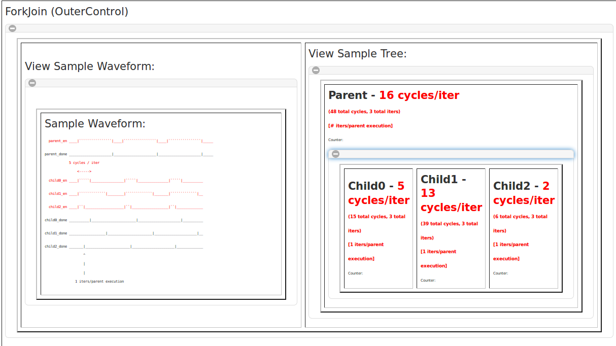
The third style is ForkJoin (OuterControl). This schedule is sometimes referred to as Parallel, because all of the children will run simultaneously with no regard for dependencies between each other. Similar to Pipelined scheduling, the only controller that matters at all in this schedule is the longest stage. Speeding up the runtime of non-critical stages will result in no speedup, since there is no transient period for this kind of controller.

The fourth style is Fork (OuterControl). These kinds of structures are generated from if-then-else statements in Spatial in cases where the condition cannot be used to predicate a primitive, nor can the node be replaced with a mux or one-hot mux. If conditional branching is used around actual control structures, such as loads, stores, or explicit controllers, a Fork will be generated. When looking at instrumentation for this kind of schedule, you should think of the cycle counts of each child as a “duty cycle” for that particular child versus the other siblings.

The fifth style is a Streaming (OuterControl). There is no associated waveform because it is tricky to demonstrate how this kind of controller works. The best way to think about this kind of controller is a ForkJoin that could have dependencies between the children. This controller is implemented the same way, except the enable of each child is anded with the ready/valid signals for all streams being read/written inside of the child. This is for data-level pipelining. It is used implicitly for DRAM loads/stores, but can also be used explicitly in an app. FIFOs and FIFORegs can be used to mediate the control flow between the stages.

Finally, there is a *** (InnerControl) example. Every leaf controller in the hierarchy is an inner controller, and they can be characterized by their latency and initiation interval (shown in the grey box). The latency describes how many cycles after the stage is enabled it will take for the last primitive in the body to execute. This describes the delay of the done signal relative to the enable signal for a controller that executes for one cycle. The initiation interval describes how many cycles the controller must wait before incrementing its counter by one step and issuing the next iteration of the body.

A third signal is included in the waveforms, which is the datapath enable signal. This signal is the boolean that is retimed and distributed to all of the nodes in the body of the controller. It is also generally used as part of the read/write enable signals to memories. Not shown in this sketch is the case of Streaming inner controllers, which behave exactly the same way except the ready signals of written streams are used as backpressure and can stall the entire dataflow inside the body and the valid signals of read streams are used as forward pressure to enable the controller.

Using instrumentation for performance

For quick reference, use the images to the right. For a closer look, please download the provided sample html here.

We will focus our attention on the MAINPIPE controller in the code provided at the top of this tutorial. As shown in the structure on the right, this is a three-stage pipeline. Its schedule is Pipelined, which means the three children will execute in a pipelined fashion. This controller runs for “1 iters/parent execution,” while its three children run for 8 iterations each with the given input arguments “64 128 128.” The top controller is directly inside the Accel, which runs once, so it is expected that the MAINPIPE will run for 1 iteration. All of the children of a controller should run for the same number of iterations per parent execution, and with tile sizes of 16, 64, and 64 and input arguments 64, 128, and 128, the M by bm par pM, N by bn par pN is expected to run 4x2=8 times.

The key idea here is that the middle stage, which is the one performing all of the computation on the fetched tiles, is the bottleneck for this app. It is two orders of magnitude slower than the load or store stages, so the developer should spend the most time working on this stage. By zooming in to sub-trees within this controller, the developer can see which stages should be parallelized by more, or pipelined more heavily. Often, tweaking the innermost controllers yields the greatest benefit when they have initiation intervals that are greater than 1. It is important for the user to understand why the compiler detected a loop-carry dependency cycle in the body of that controller and figure out how to eliminate it.

Another thing the developer should try is to minimize the total number of inner controllers. If possible, the code will perform better when there is one, fat inner controller, rather than a wide outer controller with lots of children. Even when the parent is pipelined, the computation in one inner controller is totally walled-off from the computation of the other controllers. Fully pipelining all of the computation in all of the leaf nodes is much more efficient, although potentially more confusing to the user, than having wide outer controllers.

It is also important to watch the initiation interval when doing this. If the initiation interval expands to consume the total latency of the longest child node in the original design, the benefits of pipelining the primitives will be lost.

using instrumentation for resource utilization

For quick reference, use the images to the right. For a closer look, please download the provided sample html here.

Also embedded in the controller hierarchy is information about all of the memories instantiated in the app. You can see the “NBuf Mems” and “Single-Buffered Mems” in boxes below the controller hierarchy. The entries in these two boxes are roughly sorted by the “cost” of each memory, so when trying to cut back on resources, you should pay more attention to those at the top of this list. Each entry contains details about that particular memory, including volume for a single buffer, number of buffers, padding, banking, and whether there are cross-bar reads or writes. The NBuffered memories are buffered because the compiler detected a pipelined least common ancestor (LCA) between all of the accesses. It inserted a buffer for each child of the LCA that lies between the first and last accesses. One exception is that there is support for broadcast writers, which occurs when one or more of the writers to the memory raises the LCA to a controller that has sequential scheduling. In this case, this write is sent to all buffers, and then it behaves as a buffered memory when the pipelined LCA for the subset of controllers is active. Each NBuffered memory is annotated directly in the controller hierarchy to indicate which controllers are responsible for each buffer of the memory. Each memory is assigned a random color to help the user visually trace them from controller to controller.

You may notice that some memories that you tried to create one instance of now have multiple instances. This could be due to unrolling or duplication from banking. You should use this information about memories to cut back on buffer depth where appropriate and try to avoid cross-bar connections.

The image on the right shows explicit lines connecting each buffer of each buffered memory in the example app. All memories here are double buffered, but it is possible to have more buffers in other cases.

previous: workload arbiter

next: performance (best practices)